Brainomaly: Unsupervised Neurologic Disease Detection

Utilizing Unannotated T1-weighted Brain MR Images

The paper: Brainomaly: Unsupervised Neurologic Disease Detection Utilizing Unannotated T1-weighted Brain MR Images

Hello everyone!

Today, we’re diving into the intriguing topic of brain health and one of its cutting-edge techniques: anomaly detection in brain imaging. While the topic might sound complex at first, I assure you we’ll navigate it together step by step.

When it comes to understanding the brain, we have a variety of tools at our disposal: CT scans, MRIs, PET scans, mammograms, ultrasounds, X-rays, and more. These tools aren’t just fancy names; they play a crucial role in helping us see inside the brain, highlighting potential issues and conditions. Our goal? Spotting problems early, ensuring accurate diagnoses, and providing effective treatments.

These anomalies, or deviations, can often be early signs of health changes. Recognizing them promptly can lead to better care and a deeper understanding of potential health concerns.

Guiding us through this intricate process is technology. Techniques like convolutional neural networks (CNNs) offer detailed views, while autoencoders help identify these deviations. And let’s not forget about GANs, they assist in visualizing and understanding these complex brain patterns. But beyond the technicalities, each anomaly carries its own unique story. By uncovering and understanding these stories, we gain valuable insights into the broader landscape of brain health and its intricacies.

Are you intrigued? Let’s dive deeper into the fascinating world of brain imaging and the stories behind each anomaly.

Unraveling Brain Imaging: The Roadblocks Ahead

Brain imaging, an area where science meets art, presents its own set of hurdles, especially when delving into anomaly detection. Lets break down the core challenges we face in this captivating domain.

1. The Quest for Quality Brain Scans

At the heart of any machine learning project lies data. In the world of brain imaging, this data is not just any data—it’s the intricate patterns of our brain. Achieving high-quality brain scans is no small feat. Special equipment is essential, and the process demands the keen eye of experts to meticulously label each detail. With supervised learning, where every image needs annotation, the sheer volume required can be daunting.

The intricacies of annotating brain images can’t be overstated. It’s a meticulous task that demands expertise and patience. As we push the boundaries, aiming to capture more dynamic aspects of brain function, the challenge of acquiring and annotating data only grows.

2. Embracing New Learning Techniques

Given the complexities of manual annotation, there’s a growing shift towards exploring unsupervised and semi-supervised methods in brain imaging. While traditional supervised approaches have their place, the evolving landscape of brain imaging calls for more adaptable and efficient techniques.

Unraveling Anomalies: The Delicate Balance with Medical Data

“It’s in the anomalies that nature reveals its secrets.” ― Johann Wolfgang von Goethe

In the complex landscape of medical data, anomalies act as subtle indicators of the unexpected. These deviations, though nuanced, can reveal critical insights, particularly in patient care and diagnosis. Let’s explore the significance and techniques of anomaly detection within medical datasets.

A Closer Look at Anomalies: A Medical Perspective

Anomaly detection in medical data serves as a vigilant guard, ensuring that no irregularity remains unnoticed. Imagine this: Among numerous routine MRI scans depicting typical brain structures, one scan presents a distinctive pattern—perhaps an unusual concentration of neural activity or an atypical tissue formation. Such anomalies could hint at early-stage conditions or previously unrecognized physiological phenomena.

Here’s a glimpse into the varied applications of anomaly detection in the medical context:

• Diagnostic Imaging: Detecting irregularities in MRI, CT, or X-ray images that may indicate potential health issues.

• Patient Monitoring: Continually analyzing patient metrics and vitals to spot sudden or gradual deviations that may warrant attention.

• Drug Efficacy: Monitoring patient responses to medications to identify any unexpected reactions or side effects.

• Genomic Sequencing: Recognizing unexpected patterns or sequences within genetic data that could point to genetic anomalies or mutations.

• Clinical Trials: Scrutinizing data from experimental treatments to highlight any unforeseen responses or outcomes.

The incorporation of anomaly detection in the medical context emphasizes its essential role in enhancing patient care and driving medical advancements.

Anomaly Detection: Tools and Strategies

Effectively navigating the intricacies of medical data necessitates a combination of robust methodologies and advanced techniques. Here’s an overview of the methodologies and tools utilized in anomaly detection within medical datasets:

• Statistical Methods: Using fundamental statistical metrics to identify deviations in patient metrics or imaging data from established standards.

• Machine Learning Models: Harnessing algorithms like One-Class SVM and Isolation Forest to analyze extensive datasets and flag potential anomalies in patient information or diagnostic images.

• Deep Learning Techniques: Employing deep neural networks, particularly convolutional neural networks (CNNs), Autoencoders or GANs to scrutinize detailed patterns in medical images and highlight subtle irregularities.

• Time-Series Analysis: Applying temporal data analysis techniques to monitor patient vitals and metrics over time and detect deviations from anticipated patterns.

• Ensemble Methods: Merging multiple detection models to amplify accuracy and reliability, ensuring thorough examination of medical data.

In conclusion, anomaly detection within medical data stands as a foundational pillar of contemporary healthcare, fostering early detection, tailored treatment, and innovative research.

Understanding Anomaly Detection in Healthcare

In the area of healthcare, detecting anomalies is crucial. This section offers insights into the methods and strategies used in medical anomaly detection, emphasizing the unique challenges and solutions within the healthcare domain.

• Mapping Anomalies with Supervised Techniques Within the medical sphere, supervised methods hinge on datasets where patient outcomes guide algorithmic learning. By assimilating clinical data, these techniques aim to pinpoint deviations from typical patient profiles. However, given the diverse nature of health anomalies and the ever-evolving medical landscape, there’s a constant need for models that can adapt and discern novel irregularities.

• Uncharted Patterns with Unsupervised Strategies Unsupervised methods in healthcare, sifting works without predefined labels. They excel at identifying patterns, yet the challenge lies in discerning genuine anomalies from benign fluctuations. Their strength, however, lies in their ability to uncover unexpected insights, potentially leading to breakthroughs in patient care.

• The Hybrid Approach: Harnessing the Power of Semi-supervised Methods Combining the best of both worlds, semi-supervised strategies tap into extensive unlabeled datasets, complemented by sparse labeled samples. These models can then be fine-tuned using specialized datasets, ensuring precision in detecting anomalies that truly matter.

Within our research context, we turn our attention to unsupervised methods. While their approach is exploratory, it’s this very exploration that might uncover novel insights, making them indispensable for understanding the nuances of healthcare anomalies.

Detecting Unusual Patterns by Understanding the Typical

Most methods for spotting anomalies start by understanding what’s normal. Then, they use this understanding to spot anything unusual. This method is often linked with certain learning techniques and has two main steps.

First, a model of regular behavior is created using the data available. Depending on the method used, this data might include just regular examples or a mix of both regular and unusual ones. After this model is set, each piece of data gets a score based on how different it is from the norm.

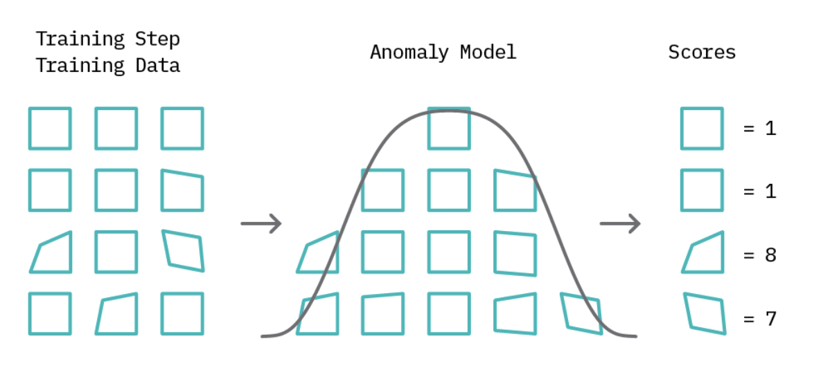
In the second part of spotting unusual data, we set a limit called a “threshold.” For instance, if a score surpasses this set threshold, it’s labeled as an anomaly; otherwise, it’s classified normal. This threshold concept giving analysts a straightforward tool to adjust the precision of anomaly detection. Although many anomaly detection techniques use this foundational idea, their approaches diverge in how they define typical patterns and calculate anomaly scores.

Brainomaly: Detecting Neurological Anomalies

After getting into the basics of anomaly detection and the important role of thresholds, we can have closer look at the Architecture of Brainomaly.

Brainomaly’s architecture hinges on two foundational networks:

-Discriminator Network: This network, rooted in the PatchGAN architecture, determines the authenticity of T1-weighted brain MRIs. Its task? To discern between real MRIs and those generated by the system.

-Generator Network: Operating on the encoder-decoder principle, this network dives deep into the MRI data, taking T1-weighted brain MRIs as input. Unlike traditional models, it doesn’t aim to recreate the entire image. Instead, it crafts additive maps highlighting the changes needed to transform a given brain into a healthy state. The magic happens when this map is combined with the input MRI, resulting in a synthesized healthy-brain MRI.

Generative Adversarial Networks (GANs):

So lets delve deeper into the advancements of artificial intelligence,into a concept that stands out for its innovation and transformative potential: Generative Adversarial Networks, commonly known as GANs. Introduced by Goodfellow and his team in 2014.

At its foundational level, a GAN operates on a bilateral framework, characterized by two primary components: the “generator” and the “discriminator.” The generator is tasked with a remarkable challenge—it endeavors to produce synthetic samples that are indistinguishable from real data. This concept simulate a compelling duel between these two neural networks.

Unraveling GANs in Medicine: Bridging Data Gaps with Generators and Discriminators

In the complex area of medical research and diagnosis, Generative Adversarial Networks (GANs) are making waves. Imagine a medical lab where one part creates artificial medical images, while another part carefully checks them to ensure they look genuine and reliable.

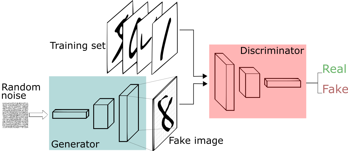
The Medical Detector: Generator and Discriminator

Generator (G)

• Probabilistic Mapping: Envision a generative model $G$ that transforms a latent variable $z$ from a prior distribution $p_z(z)$ into intricate medical images, striving to mirror the authentic data distribution $p_{data}(x)$
• Mathematical Insight:
  • Input: $z \sim p_z(z)$
  • Output: $G(z) \sim p_{data}(x)$

Discriminator (D)

• Clinical Scrutiny: The Discriminator $D$ functions as a binary classifier, estimating the probability $D(x)$ that a given medical image $x$ is derived from genuine patient data $p_{data}(x)$.
• Mathematical Representation:
  • Input: $x$
  • Output: $D(x) \in [0, 1]$

Probabilistic Objective Function: Deciphering Authenticity

Central to the GAN architecture is the probabilistic objective function, quantifying the adversarial dynamics:

• Clinical Validity: The first term $E_{x \sim p_{data}(x)}[\log D(x)]$ gauges the expected log likelihood of the Discriminator correctly identifying genuine medical images.
• Synthetic Analysis: The second term $E_{z \sim p_z(z)}[\log(1 - D(G(z)))]$ measures the anticipated log likelihood of the Discriminator discerning synthetic images produced by the Generator.

Iterative Training Dynamics: Convergence towards Diagnostic Excellence

1. Generator: The Generator creates fake medical images, using some random input $z$.
2. Discriminator: The Discriminator carefully checks both real and fake images, getting better at telling them apart.
3. Over time, both the Generator and Discriminator get so good that the fake images look almost real, and the Discriminator becomes really good at spotting any differences.

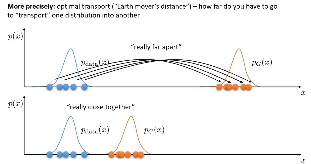
The Wasserstein Innovation

Theres on last step missing to understand the Equation in our paper. Traditional GANs, despite their prowess, sometimes wrestle with specific issues such as training instabilities and the daunting “mode collapse.This phenomenon restricts the Generator, causing it to produce a limited repertoire of images, thereby undermining the breadth and diversity of the synthetic data. Like an artist stuck in a creative loop. WGANs, or Wasserstein GANs, change the game. They offer a broader range of outputs using a mathematical measure called the Wasserstein distance, ensuring diversity and quality.

This is precisely where the innovation of Wasserstein GANs (WGANs) shinesshos their advantage. By introducing the Wasserstein distance, WGANs address some of the foundational limitations of their predecessors.

The Math Unveiled

At its core, the Wasserstein distance quantifies the difference between two probability distributions. In the context of GANs, it acts as a more reliable measure, enabling smoother gradients and thereby facilitating more consistent training.

The Core WGAN Objective

At the heart of WGANs is the Wasserstein distance, which serves as the guiding metric for the model’s optimization. The objective function of WGANs is expressed as:

\(\min_{G} \max_{D \in \mathcal{D}} \mathbb{E}_{x \sim p_{\text{data}}(x)}[D(x)] - \mathbb{E}_{z \sim p_{z}(z)}[D(G(z))]\) This equation essentially aims to minimize the difference between the distributions of real and generated data.

The Role of Gradient Penalty

To further enhance stability and ensure specific constraints on the discriminator’s behavior, a gradient penalty term is introduced. This term is vital for enforcing the Lipschitz constraint, a mathematical property that guarantees the stability of the model.

The gradient penalty term is represented as:

Here, $\lambda$ acts as a regularization parameter, controlling the intensity of the penalty, and $\hat{x}$ represents samples drawn along straight lines between real and generated data points.

Integrating the Gradient Penalty

Merging the original WGAN objective with the gradient penalty, we get a comprehensive objective function:

The Advantages of Incorporating Gradient Penalty

1. Stability Boost: The gradient penalty acts as a stabilizing force, reducing the likelihood of training pitfalls like mode collapse.
2. Quality Enhancement: With a smoother discriminator, WGANs produce more refined and high-quality outputs.
3. Theoretical Grounding: The gradient penalty brings WGANs closer to theoretical guarantees, ensuring reliable convergence under specified conditions.

Understanding the Mechanics of Brainomaly: The Additive Map and the Tanh Function

Brainomaly represents a groundbreaking fusion of advanced mathematics and medical imaging. Central to its operation are two key components: the additive map and the tanh activation function. Let’s delve into their roles and significance.

The Additive Map: Making Brain Scans clearer

We almost understand the special math behind Brainomaly, a tool that helps doctors see brain issues better. Let’s dive into what makes the trick. In Brainomaly’s architecture, the generator doesn’t directly craft a full healthy-brain MRI. Instead, it formulates an “additive map.” Visualize this map as a meticulous set of instructions. For every voxel (essentially a 3D pixel) in the original brain MRI, this map outlines the necessary adjustments required to transition the brain to a healthy state. The additive map in the Brainomaly method represents the estimated required changes for each voxel in a T1-weighted brain MRI to transform it into a healthy brain MRI. Let’s break down this concept with a simple matrix example.

Consider an original brain MRI represented by the matrix $A$: \(\begin{bmatrix} a & b \\ c & d \end{bmatrix}\)

The additive map, denoted as $M$, is another matrix indicating the required changes: \(\begin{bmatrix} 0.1 & 0.2 \\ 0.3 & 0.4 \end{bmatrix}\)

The final healthy-brain MRI is generated by element-wise addition of $A$ and $M$:

The additive map is a crucial component in the Brainomaly method, providing insights into the changes required to transform a given brain MRI into a healthy state. This innovative approach showcases the potential of unsupervised learning for neurologic disease detection.

The Role of Tangent Hyperbolic (tanh)

Once crafted, the additive map is combined with the original MRI to produce the final healthy-brain MRI. Mathematically, this fusion involves a voxel-wise summation:

The tanh function—short for tangent hyperbolic—plays a crucial role here. This mathematical tool maps its input to a value between -1 and 1. By applying the tanh function to the combined MRI and additive map, the structural coherence and quality of the resulting image are preserved, ensuring clinically relevant outputs. Brainomaly uses a special equation to make sense of brain pictures. This equation is like a magic recipe that combines math with real brain images to spot health problems.

We’ve Reached the Core Equation!

After all our work, we’ve landed on Brainomaly’s main equation:

This equation is at the heart of how Brainomaly works.

CreatingMedical Precision: Brainomaly’s Training Methodology

In the intricate choreography of Brainomaly’s training process, the interplay between real and synthetic brain images is pivotal. Let’s look into the essential steps, sh the systematic progression that shapes this unsupervised neurologic disease detection model.

Step 1: Discriminator’s Diagnostic Prowess (Real Loss)

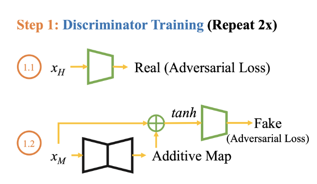
1.1 Healthy Data

• Objective: Train the discriminator to recognize real brain images from healthy subjects ($x_H$).
• Real Loss Component: Assess how well the discriminator can distinguish genuine brain scans in a healthy dataset. \(LD_{adv1} = E_{x \sim H} [D_{real/fake}(x_H)]\)

1.2 Mixed Data

• Objective: Further refine the discriminator’s ability by exposing it to a mixed dataset containing brain images from individuals with neurologic diseases and healthy subjects.
• Real Loss Component: Evaluate the discriminator’s performance in distinguishing real brain scans within the mixed dataset. \(LD_{adv2} = [D_{real/fake}( \text{tanh}(x_M + G(x_M)))]\)

Step 2: Generator’s Medical Artistry (Adversarial and Identity Loss)

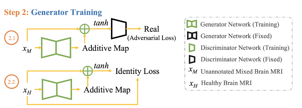
2.1 Adversarial Loss with Mixed Data

• Objective: Task the generator with creating brain images ($G(x_M)$) that are indistinguishable from real ones, even in the mixed dataset.
• Adversarial Loss ($LG_{adv}$): Assess how well the generator fools the discriminator in the mixed dataset. \(LG_{adv} = - E_{x \sim M} [D_{real/fake}(\tanh(x_M + G(x_M)))]\)

2.2 Identity Loss with Healthy Data

• Objective: Preserve unique features in the generated images to maintain authenticity.
• Identity Loss Component: Ensure that the generator doesn’t lose its ability to accurately reproduce specific details in healthy brain images. \(L_{id} = E_{x \sim H} [||G(x_H) - x_H||_1]\)

2.3 Full Generator Ensemble

• Objective: Harmonize adversarial and identity losses for a balanced and clinically relevant performance.
• Full Generator Ensemble ($LG$): Combine adversarial and identity losses with appropriate weights. \(LG = LG_{adv} + \lambda_{id} L_{id}\)

Iterative Refinement: A Symphony of Improvement

During the iterative refinement process, both the discriminator and generator enhance their abilities through exposure to various datasets.

At the end of training, Brainomaly achieves a harmonious balance between the discriminator’s ability to distinguish real from synthetic scans and the generator’s skill in crafting neurologically significant images.

Finally, Brainomaly is finely tuned—a discriminator with sharpened diagnostic precision and a generator crafting clinically relevant brain imagery.

Step 3: Testing Brainomaly with Mixed Input Data - An Illustrated Example

Understanding the Diverse Datasets

Before we dive directly into the testing phase, it’s essential to grasp the composition of the datasets it encounters. Brainomaly engages with two distinct datasets:

1. Alzheimer’s Disease Dataset: Navigating Complexity

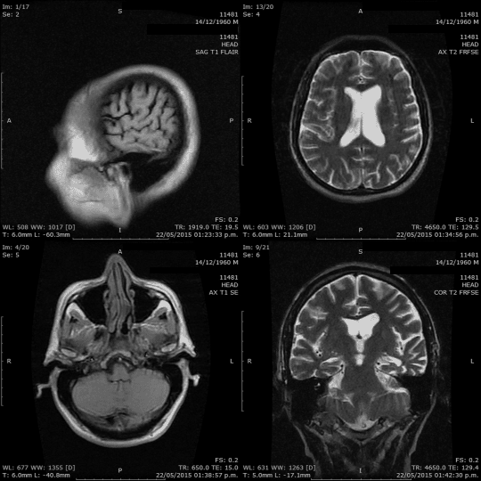
   Brainomaly explores the intricacies of the Alzheimer’s disease dataset. This dataset comprises a mix of T1-weighted brain MRIs from healthy controls and patients with Alzheimer’s disease. It provides a rich landscape for Brainomaly to showcase its ability to discern subtle structural changes indicative of neurologic diseases.

2. Headache Dataset: A Migraine of Challenges

   Additionally, Brainomaly confronts a diverse headache dataset. This collection includes MRIs from individuals with migraine, acute post-traumatic headache (APTH), and persistent post-traumatic headache (PPTH), diagnosed according to the International Classification of Headache Disorders (ICHD). The varied nature of this dataset poses unique challenges, allowing Brainomaly to prove its adaptability in diagnosing different neurologic conditions.

Now, Let’s Walk Through the Testing Process

With a solid understanding of the datasets at hand, let’s illustrate how Brainomaly tackles the testing phase using an example from the Alzheimer’s disease dataset.

A Practical Medical Example: Alzheimer’s Disease

Imagine presenting Brainomaly with a T1-weighted brain MRI from an individual diagnosed with Alzheimer’s disease. In this scenario, the generator within Brainomaly undertakes a meticulous task — crafting an image that mirrors the structural patterns of a healthy brain while subtly accentuating the disease-specific alterations.

The generated image, resembling that of a healthy brain, undergoes a critical evaluation. Brainomaly meticulously examines the difference between the generated and original images, creating what is known as a difference map. This map, in essence, highlights structural changes, offering insights into the specific nuances associated with Alzheimer’s disease.

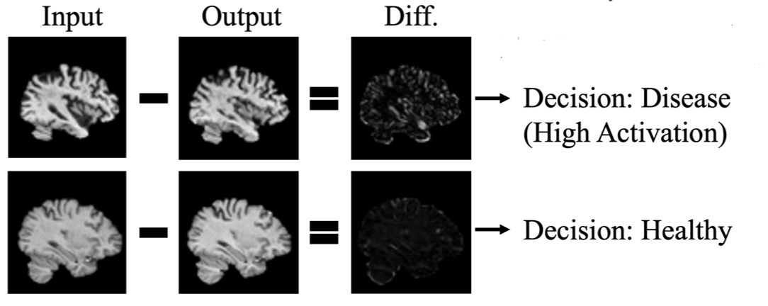
Within this difference map, activated regions emerge — these are voxels signaling structural shifts that could be indicative of neurologic anomalies. The culmination of these activations contributes to the computation of a disease detection score. A higher disease detection score signifies a heightened likelihood of the input brain MRI bearing the hallmarks of Alzheimer’s disease.

Decoding Brainomaly’s Methodology: Key Components

1. Dataset Composition:
   • A blend of T1-weighted brain MRIs, featuring both healthy and Alzheimer’s-afflicted individuals.
2. Generator’s Discriminative Power:
   • The generator crafts images resembling healthy brains while preserving disease-specific alterations.
3. Difference Maps:
   • The subtraction of generated healthy brain MRIs from the originals creates difference maps.
4. Disease Detection Scores:
   • Activations within these maps contribute to the calculation of disease detection scores.
5. Pseudo-AUC Metric:
   • In the absence of annotated samples, Brainomaly relies on the Pseudo-AUC metric for model selection.

A Closer Look at AUC

As Brainomaly concludes its testing phase, the evaluation becomes crucial in comprehending its diagnostic prowess. The Area Under the Curve (AUC) provides a nuanced measure of the model’s ability to distinguish between healthy and diseased cases.

Understanding AUC in Medical Terms:

AUC quantifies the model’s ability to rank the disease detection scores — a higher AUC indicates a more accurate discrimination between healthy and neurologically compromised brains. In scenarios where annotated samples are scarce, the Pseudo-AUC metric steps in. Brainomaly leverages this metric to select the model with the highest AUCp for inference.

As Brainomaly unfolds its diagnostic capabilities, the combined prowess of its methodology and evaluation metrics establishes it as a robust ally in the diagnosis of unsupervised neurologic disease detection.

Results and Impact

Understanding Brainomaly’s Experiments: Unraveling Neurologic Disease Detection

Let’s examine further the intricacies of Brainomaly’s experiments, a scientific collaboration with Mayo Clinic aimed at advancing neurologic disease detection.

The Foundation: Diverse Data Integration

To grasp Brainomaly’s capabilities, starts with the integration of diverse data. Mayo Clinic’s collaboration introduces MRIs from 428 healthy controls, enriched with various headache types. This strategic diversity mirrors real-world scenarios, challenging Brainomaly to discern patterns across distinct neurologic conditions.

The methodology initially grouping all headache types together. This deliberate step provides Brainomaly with a holistic understanding before delving into the specifics of each subtype. The goal is to equip the model with the capability to decode varied neurologic signatures effectively. HEAD DS1 and HEAD DS2 – are comprising unannotated mixed brain MRI sets. Balanced with representations of migraine, APTH, and healthy controls, these sets serve as proving grounds for Brainomaly’s capabilities. By aggregating slice-level predictions and delving into patient-level evaluations, the analysis gains depth.

Navigating Transductive and Inductive Learning

Brainomaly showcases its impressive adaptability by seamlessly maneuvering through both transductive and inductive learning scenarios. During training, it adeptly handles an unannotated mixed brain MRI set, demonstrating its prowess in transductive learning. Additionally, in the inductive learning setting, Brainomaly confidently applies its insights to an unseen test set.

Unraveling Neurologic Disease Detection: Brainomaly’s Experiment Results

Now that we’ve delved into the intricacies of Brainomaly’s experiments, let’s uncover the results that showcase its prowess in neurologic disease detection.

A Closer Look at Alzheimer’s Disease Detection

In the recognition of Alzheimer’s disease detection, Brainomaly stands out with an average AUC of 0.6550. Comparing this with six state-of-the-art methods, Brainomaly outperforms the competition by a significant margin. Even against the best-performing method, f-AnoGAN, Brainomaly exhibits an 8.09% improvement.

Illuminating Headache Detection Insights

Transitioning to headache detection, Brainomaly continues to perform. With an impressive average AUC of 0.8960, it outperforms competitors like HealthyGAN, ALAD, Ganomaly, and DDAD. HealthyGAN, the closest contender, lags behind by 13.84%, highlighting Brainomaly’s superior ability to detect various headache subtypes.

Digging deeper into sub-type detection, Brainomaly demonstrates precision. In migraine detection, it achieves a precision of 0.9375 with only 3 misclassifications out of 48. For APTH detection, the precision is 0.3750 (15 incorrect out of 24), showcasing the method’s room for improvement in this particular category. However, in PPTH detection, Brainomaly excels with a precision of 0.9600, making only 1 incorrect classification out of 25.

Validating the AUC Metrics

The AUC metrics used for evaluation, both in Alzheimer’s disease and headache detection, underscore Brainomaly’s effectiveness. Not only does it outperform existing methods, but it also exhibits consistency in its performance across different scenarios and subtypes.

Future Horizons

As we examine the results, it’s evident that Brainomaly is not just a solution for today’s challenges but a promising avenue for future exploration. Its robust performance in diverse scenarios positions it as a frontrunner in the area of unsupervised neurologic disease detection.

In conclusion, the results affirm Brainomaly’s potential to redefine medical imaging boundaries, offering a glimpse into a future where unsupervised methods play a pivotal role in disease detection.

Future Directions and Challenges

Advancements in Anomaly Detection

Briefly touch upon potential advancements and trends in anomaly detection research.

Exploring the Idea of Stable Diffusion in Brainomaly

By steppig deeper into Brainomaly’s GAN-driven methodology, my musings led me to an intriguing idea—what if we introduced stable diffusion into this innovative mix? It’s not about questioning the triumphs of GANs but rather about exploring how an additional layer, like stable diffusion, might elevate Brainomaly’s prowess in neurologic disease detection.

As we navigate the nuances of image generation, GANs have rightfully earned their reputation for intricate detailing. However, the quest for detail sometimes ushers in fluctuations. Enter stable diffusion—an elegant alternative in my eyes. It promises a delicate touch, refining precision and infusing stability into the generated images.

Acknowledging GANs’ achievements, it’s essential to address their Achilles’ heel—mode collapse. Here’s where my ponderings take a turn. I see stable diffusion as a potential savior, injecting a broader array of features that could fortify the robustness and adaptability of Brainomaly in detecting neurologic diseases.

This isn’t a call to replace GANs; it’s more like introducing a companion that complements and streamlines, contributing to a more efficient neurologic disease detection methodology.

Consider the uncharted territories of unannotated mixed brain MRI sets. Here, stable diffusion could play a pivotal role, smoothing transitions between different data distributions. This excites me, especially in transductive learning settings, where Brainomaly thrives in adapting to diverse scenarios.

My Personal Invitation to Innovation

In essence, my take on integrating stable diffusion into Brainomaly isn’t just an abstract idea—it’s a personal invitation to explore uncharted dimensions. It’s about enriching an already powerful methodology with refined precision, enhanced adaptability, and a touch of computational elegance.

As I draw my conclusions, I see this contemplation as a small step toward a future where innovation and personal ideas converge. It’s about contributing a thread to the rich tapestry of medical imaging, unlocking new possibilities in understanding and diagnosing neurologic diseases.

References

[Charu C. Aggarwal]. (Outlier Analysis,Second Edition). Springer International Publishing AG ,2017

Computer vision and machine learning for medical image analysis: recent advances, challenges, and way forward, 2022

Deep Learning for Anomaly Detection: A Review, 2020

Machine Learning & Deep Learning Techniques for Anomaly Detection in Medical Imaging,2023

A Comprehensive Introduction to Anomaly Detection, 2023

Anomaly Detection Wikipedia

Deep Learning for Anomaly Detection, 2020

From GAN to WGAN , 2017