Title: Implementing a deep Q-learning algorithm based on the paper “Human-level control through deep reinforcement learning” by David Silver et al.

The paper: Human-level control through deep reinforcement learning

The code of this project can be found at

Before we implement the DQN Network for the Atari game let’s have look at the first DQN paper. The quest for artificial intelligence (AI) capable of human-level performance has long captivated researchers. One significant milestone in this journey was the groundbreaking paper “Human-level control through deep reinforcement learning” by David Silver and his colleagues, which was published in 2015. This seminal work introduced a novel approach to reinforcement learning (RL) that enabled AI to achieve unprecedented levels of performance in complex environments, particularly in the realm of video games.

The Challenge: Bridging the Gap Between AI and Human Performance

Before Silver’s work, AI systems struggled to perform at a level comparable to humans in tasks requiring nuanced decision-making and adaptability. Traditional reinforcement learning methods were limited in their ability to process high-dimensional sensory inputs, such as the pixels of a video game screen, and to learn effective policies directly from these inputs. The challenge was to create an AI that could not only perceive its environment with human-like fidelity but also make decisions and take actions that lead to optimal outcomes.

The Solution: Deep Q-Networks (DQNs)

David Silver and his team at DeepMind proposed a solution that combined deep learning with reinforcement learning, resulting in the Deep Q-Network (DQN). The DQN architecture utilized a convolutional neural network (CNN) to process raw pixel input from the environment, extracting useful features automatically. This representation was then fed into a Q-learning algorithm, a type of reinforcement learning that aims to learn the value of taking certain actions in specific states to maximize cumulative rewards.

Q-Learning and Bellman Equation

At the heart of Q-learning is the Q-function, ( Q(s, a) ), which estimates the expected future rewards of taking action ( a ) in state ( s ). The Q-function is updated using the Bellman equation:

where:

• $( s_t )$ and $( a_t )$ are the state and action at time $( t )$
• $( r_t )$ is the reward received after taking action $( a_t )$
• $( \alpha )$ is the learning rate
• $( \gamma )$ is the discount factor

Deep Learning with CNNs

To handle high-dimensional input like images, DQNs use convolutional neural networks (CNNs). The CNN automatically extracts hierarchical features from raw pixel data, allowing the agent to understand the environment at different levels of abstraction. The architecture typically consists of several convolutional layers followed by fully connected layers, ultimately outputting Q-values for each possible action.

Techniques for Stable Learning

Experience Replay

One key innovation in Silver’s work was the use of experience replay. Instead of learning from consecutive frames, experiences (state, action, reward, next state) are stored in a replay memory and sampled randomly during training. This breaks the temporal correlations between consecutive samples and improves the stability and efficiency of learning.

Target Networks

Another crucial technique is the use of a separate target network, ( \hat{Q} ), which is a copy of the Q-network and is updated less frequently. This helps to stabilize learning by providing a consistent target for the Q-value updates.

Achieving Human-Level Performance

To demonstrate the effectiveness of their approach, Silver and his team tested the DQN on a suite of Atari 2600 video games. The results were astonishing: the DQN was able to outperform the best existing algorithms and, in many cases, exceed human performance. Games like Breakout, where strategic planning and precise timing are crucial, showcased the DQN’s ability to learn complex control policies directly from the raw pixel data.

Mastering Atari Games with Deep Q-Learning: An Implementation Guide

Deep Q-Learning has become a game-changer in the realm of reinforcement learning, especially for mastering complex environments like Atari 2600 games. This blog post will take you through the detailed journey of Deep Q-Learning with Experience Replay, exploring preprocessing techniques, model architecture, training intricacies, and the innovative tweaks that make this method so powerful.

Preprocessing: Simplifying the Complex

Working directly with raw frames from Atari 2600 games is computationally expensive and challenging due to the high dimensionality and color complexity. To handle this, we use some clever preprocessing steps:

Tackling Frame Flickering: MaxAndSkipEnv

In many Atari games, objects flicker due to the limited number of sprites the console can handle simultaneously. To mitigate this issue, we utilize the MaxAndSkipEnv wrapper. This wrapper selects the maximum value for each pixel color over the current and the previous frame. By doing so, it stabilizes the visual input seen by the agent, providing a consistent view of the game environment.

Simplifying Color Information: PreprocessFrame

Instead of using the full RGB spectrum, we extract the luminance (brightness) channel from each frame. This reduction in color complexity helps streamline the learning process while retaining essential information about the game state. Additionally, the frames are rescaled to a smaller size of 84x84 pixels. This resizing not only reduces input dimensionality but also focuses computational resources on the most relevant visual features.

Capturing Temporal Information: BufferWrapper

Understanding the game’s state over time is crucial for effective decision-making in reinforcement learning. To capture temporal dependencies, we stack the last four preprocessed frames. This results in an input size of 84x84x4, where the neural network can learn from a sequence of images rather than a single snapshot. The BufferWrapper facilitates this frame stacking process, ensuring that the agent receives coherent temporal information during training.

Converting to PyTorch Tensor: ImageToPytorch

To integrate seamlessly with PyTorch, the frames are converted into PyTorch tensors. This conversion allows for efficient computation on GPUs and leverages PyTorch’s capabilities for deep neural network training.

Normalizing Frame Values: ScaledFloatFrame

Finally, to further stabilize and normalize the input data, the frames are converted into floating-point values within the range [0, 1]. This normalization step ensures consistent and predictable data ranges for the neural network, facilitating more stable and efficient training.

Implementation Example

Here’s how these preprocessing steps can be combined in Python code:

import gym
from wrappers import MaxAndSkipEnv, FireResetEnv, PreprocessFrame, ImageToPytorch, BufferWrapper, ScaledFloatFrame

def create_atari_env(env_name, render_mode=False):
    env = gym.make(env_name, render_mode=render_mode)
    env = MaxAndSkipEnv(env, skip=4)          # Tackles frame flickering
    env = FireResetEnv(env, fire_reset=False)
    env = PreprocessFrame(env, shape=(84, 84, 1))  # Simplifies color information and rescales
    env = ImageToPytorch(env)                # Converts frames to PyTorch tensors
    env = BufferWrapper(env, buffer_size=4)  # Captures temporal information by stacking frames
    env = ScaledFloatFrame(env)              # Normalizes frame values
    return env

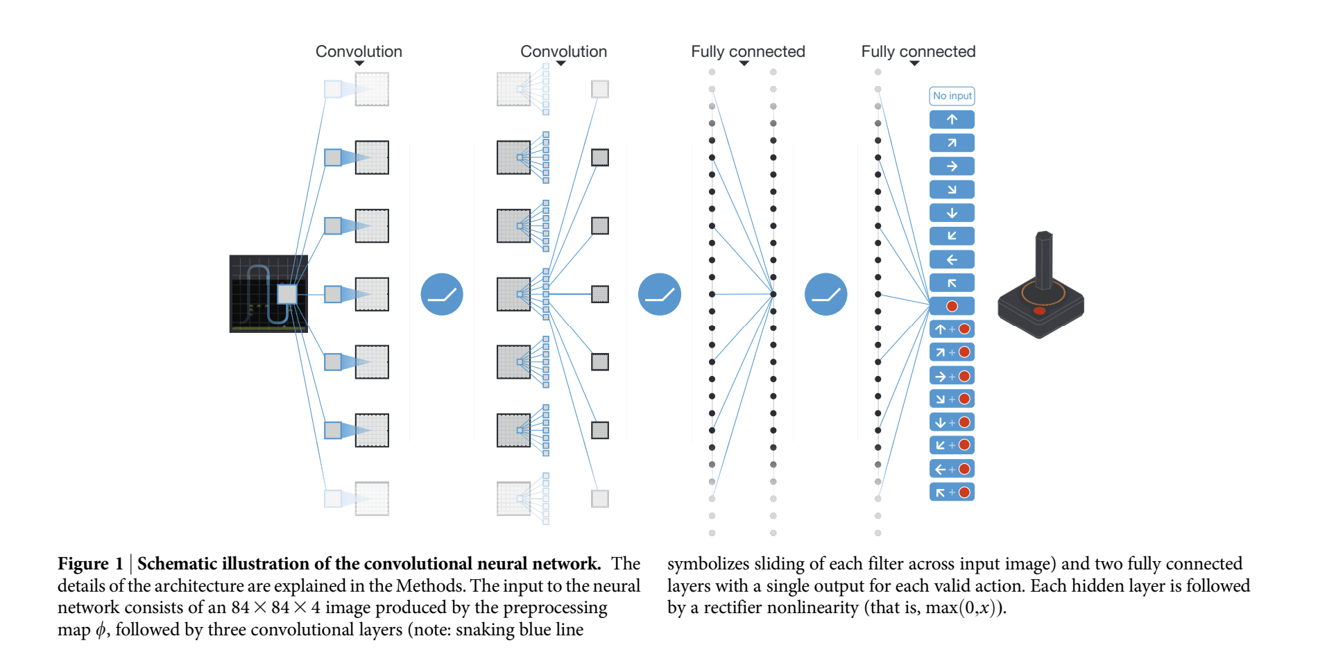
Building the Neural Network

Our deep Q-network (DQN) needs to process high-dimensional inputs and output Q-values for all possible actions efficiently. Here’s how we build it:

Input Layer

The input is an 84x84x4 image generated from our preprocessing steps.

Convolutional Layers

• First Layer: Applies 32 filters of size 8x8 with a stride of 4, followed by a ReLU activation.
• Second Layer: Applies 64 filters of size 4x4 with a stride of 2, again followed by a ReLU activation.
• Third Layer: Applies 64 filters of size 3x3 with a stride of 1, followed by ReLU.

Fully-Connected Layers

• First Fully-Connected Layer: 512 neurons with ReLU activation.
• Output Layer: Neurons equal to the number of possible actions, each representing a Q-value for that action.

Implementation Example

class DQN(nn.Module):
    def __init__(self, input_shape, num_actions):
        super(DQN, self).__init__()
        self.conv = nn.Sequential(
            nn.Conv2d(input_shape[0], 32, kernel_size=8, stride=4),
            nn.ReLU(),
            nn.Conv2d(32, 64, kernel_size=4, stride=2),
            nn.ReLU(),
            nn.Conv2d(64, 64, kernel_size=3, stride=1),
            nn.ReLU()
        )
        # Calculate the output size of the last convolutional layer
        conv_out_size = self._get_conv_out(input_shape)
        
        self.fc = nn.Sequential(
            nn.Linear(conv_out_size, 512),
            nn.ReLU(),
            nn.Linear(512, num_actions)
        )

Training the Network

Reward Clipping

Game rewards can vary wildly, making training unstable. By clipping rewards to a range of -1 to 1, we standardize the learning process and avoid issues with large gradients.

clipped_reward = np.clip(reward, -1.0, 1.0)

Exploration with Epsilon-Greedy Policy

Balancing exploration and exploitation is crucial. We use an epsilon-greedy policy where the agent chooses a random action with probability $(\epsilon)$, and the best-known action otherwise. We start with $(\epsilon=1.0)$ and anneal it to 0.1 over the fisrt 150000 frames, ensuring that the agent explores sufficiently before focusing on the best-known actions.

def get_epsilon(self):
        epsilon = max(EPSILON_FINAL, EPSILON_START - self.global_step / EPSILON_DECAY_LAST_FRAME)
        return epsilon

def select_action(self, state):
        if np.random.random() < self.epsilon:
            return self.env.action_space.sample()
        else:
            state_a = np.array([state], copy=False)
            state_v = torch.tensor(state_a, dtype=torch.float32).to(device)
            q_vals_v = self.q_net(state_v)
            _, act_v = torch.max(q_vals_v, dim=1)
            return int(act_v.item())

Key Innovations in Deep Q-Learning

Experience Replay

Instead of updating the Q-function after every action, which can lead to instability due to correlated updates, we use experience replay. Here’s how it works:

• Replay Memory: Store the last $(N)$ transitions.
• Random Sampling: Sample random minibatches of transitions for training, breaking the correlation between consecutive updates and improving data efficiency.

class ReplayBuffer:
    def __init__(self, capacity):
        self.buffer = collections.deque(maxlen=capacity)
        
    def add_sample(self, state, action, reward, done, new_state):
        self.buffer.append(Experience(state, action, reward, done, new_state))
        
    def sample(self, batch_size):
        indices = np.random.choice(len(self.buffer), batch_size, replace=False)
        states, actions, rewards, dones, next_states = zip(*[self.buffer[idx] for idx in indices])
        return np.array(states), np.array(actions), np.array(rewards, dtype=np.float32), np.array(dones, dtype=np.uint8), np.array(next_states)
    
    def __len__(self):
        return len(self.buffer)

Stansard vs Prioritized Experience Replay

In our implementation, we utilized a standard replay buffer to store and sample experiences during training. Each experience was stored with equal priority, ensuring a straightforward approach to learning from past interactions.

However, in advanced reinforcement learning techniques, such as those discussed in the paper, prioritized experience replay is often employed. This technique assigns different priorities to experiences based on their perceived importance, typically measured by their temporal-difference (TD) error. Experiences with higher TD errors are sampled more frequently, allowing the agent to focus on learning from the most informative transitions.

where $( \delta_i )$ is the TD error for transition $( i )$, and $(\epsilon)$ is a small positive constant to ensure all transitions have some chance of being sampled.

Target Network for Stability

To ensure stable learning in our reinforcement learning setup, we incorporate a dedicated target network alongside the primary Q-network. This approach mitigates oscillations and divergence in Q-values, promoting more reliable training outcomes.

Why Use a Target Network?

The primary motivation behind introducing a target network lies in stabilizing the learning process. In traditional Q-learning updates, where the Q-values are updated based on the maximum Q-value of the next state, using the same network for predictions and target values can lead to instability. This instability arises because the network’s Q-values shift rapidly as it learns, causing the target values to fluctuate, which in turn can hinder convergence.

How It Works

The target network, denoted as $( Q’(s, a; \theta^{-}) )$, operates independently from the main Q-network $( Q(s, a; \theta) )$. Here’s a breakdown of its role:

Generating Stable Q-Targets

During training, the target network generates Q-learning targets $( y_j )$ based on the next state $( s_{j+1} )$ and the action that maximizes the Q-value in that state:

Where:

• $( r_j )$ is the reward obtained after taking action $( a_j )$ in state $( s_j )$,
• $( Q’(s_{j+1}, a’; \theta^{-}) )$ denotes the Q-value predicted by the target network for the next state $( s_{j+1} )$ and action $( a’ )$, with parameters $( \theta^{-} )$.

Implementation in Code

state_action_values = self.q_net(states_v).gather(1, actions_v).squeeze(-1)
next_state_values = self.target_net(next_states_v).max(1)[0]
next_state_values[done_mask] = 0.0
next_state_values = next_state_values.detach()
expected_state_action_values = next_state_values * GAMMA + rewards_v


def train(self, num_epochs): #number of epochs the target network should be updated
        for epoch in range(num_epochs):
            episode_return = self.train_epoch(epoch)
            self.update_target_network()

In this snippet:

• self.q_net(states_v) computes the Q-values for the current states using the main Q-network.
• self.target_net(next_states_v) computes the Q-values for the next states using the target network.
• next_state_values are adjusted to 0 for terminal states (done_mask).
• expected_state_action_values are then computed using the Bellman equation, incorporating rewards and discounted future Q-values.

Updating the Target Network

The target network’s parameters $( \theta^{-} )$ are updated periodically, typically less frequently than the main network, to provide a stable set of Q-learning targets throughout the training process.

def train(self, num_epochs):
        for epoch in range(num_epochs):
            episode_return = self.train_epoch(epoch)
            self.update_target_network()

By separating the Q-learning targets from the main network’s updates, the target network introduces a delay in the learning updates, smoothing out fluctuations and promoting more consistent and effective learning over time.

Clipping the Error Term

Large updates can destabilize training. To mitigate this, we clip the error term in the Q-learning update to [-1, 1], which corresponds to using an absolute value loss function for errors outside this interval. This simple tweak significantly improves stability. The loss function $( L_i(\theta_i) )$ is:

where the TD error is clipped to ensure stability.

Putting It All Together: The Deep Q-Learning Algorithm

Here’s a step-by-step guide to the complete deep Q-learning algorithm:

Algorithm 1: Deep Q-Learning with Experience Replay
Initialize replay memory D to capacity N
Initialize action-value function Q with random weights θ
Initialize target action-value function Q' with weights θ- = θ

For episode = 1 to M do
    Initialize sequence s1 = {x1} and preprocessed sequence w1 = w(s1)
    For t = 1 to T do
        With probability ε select a random action at
        otherwise select at = argmaxa Q(w(st), a; θ)
        Execute action at in emulator and observe reward rt and image xt+1
        Set st+1 = st, at, xt+1 and preprocess wst+1 = w(st+1)
        Store transition (wt, at, rt, wt+1) in D
        Sample random minibatch of transitions (wj, aj, rj, wj+1) from D
        Set yj = rj if episode terminates at step j+1
        rj + γ maxa' Q'(wj+1, a'; θ-) otherwise
        Perform a gradient descent step on (yj - Q(wj, aj; θ))^2 with respect to the network parameters θ
        Every C steps reset Q' = Q
    End For
End For

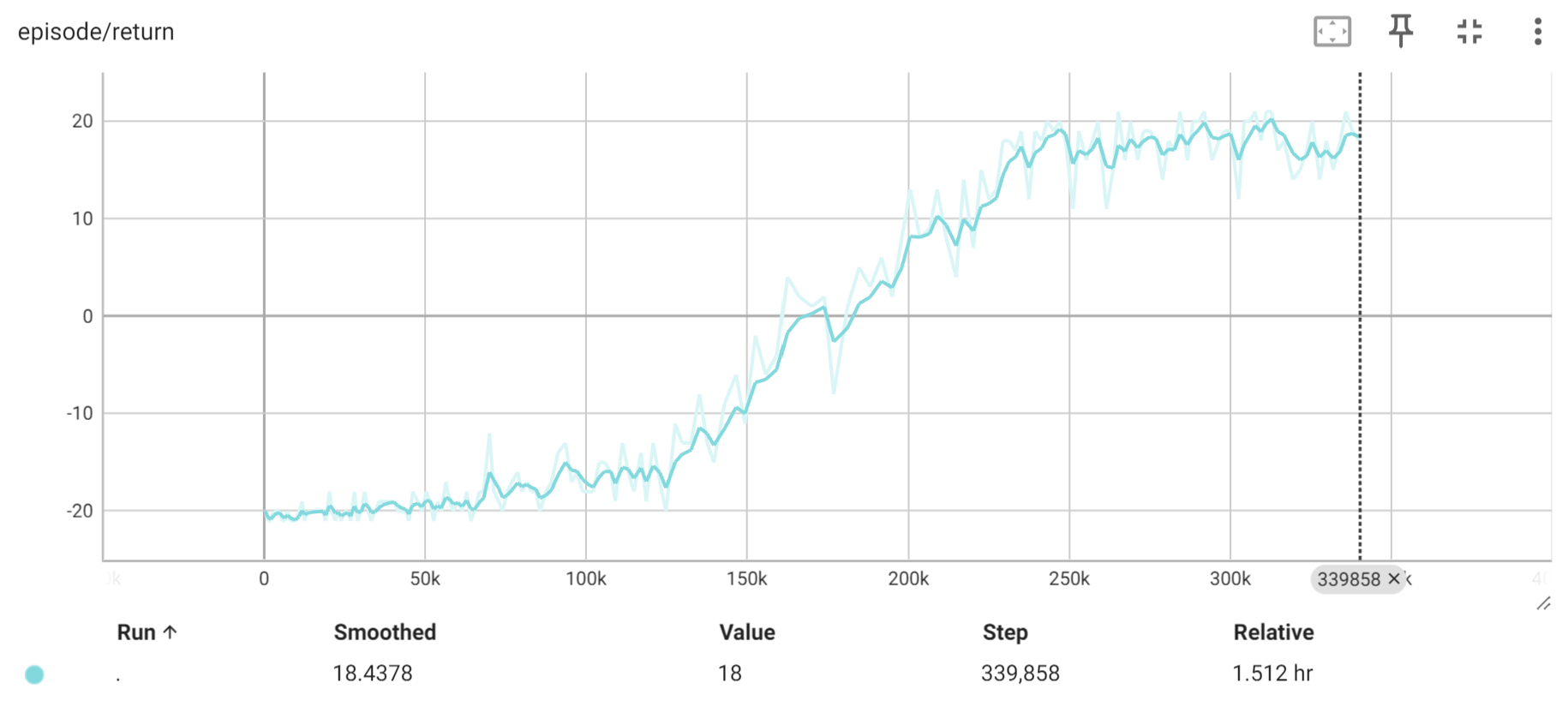
Results

After training for 200 epochs, the model has successfully converged. Here are the TensorBoard images showing the training progress:

Here is our Pong in action :)

https://github.com/SabCas/SabCas.github.io/assets/110026351/685e27f8-d6a6-47c0-8851-982a73877fd0

Improving DQN with Double Q-learning

In this post, we’ll walked through the process of training a Deep Q-Network (DQN) agent to play Atari Pong using PyTorch. Additionally, we can explore the scond paper on Double DQN, as proposed in the paper “Deep Reinforcement Learning with Double Q-learning” by Hado van Hasselt, Arthur Guez, and David Silver , can help stabilize training by addressing the overestimation bias present in standard DQN.

Standard DQN

In the standard Deep Q-Network (DQN) approach, we use a neural network to approximate the Q-values for each state-action pair. The goal is to minimize the Temporal Difference (TD) error, defined as the difference between the predicted Q-value and the target Q-value. The target Q-value is computed using the maximum Q-value of the next state from the target network:

$[ y_j = r_j + \gamma \max_a Q’(s_{j+1}, a) ]$

where:

• $( y_j )$ is the target Q-value.
• $( r_j )$ is the reward.
• $( \gamma )$ is the discount factor.
• $( Q’ )$ is the target Q-network.

The Problem with Standard DQN

One of the main issues with the standard DQN approach is the overestimation bias. Because the maximum Q-value is used for the target, it can lead to overly optimistic estimates of the action values, resulting in suboptimal policies.

Double DQN

Double DQN addresses the overestimation bias by decoupling the action selection from the action evaluation. Instead of using the maximum Q-value from the target network to compute the target, Double DQN uses the current Q-network to select the action and the target Q-network to evaluate it:

$[ y_j = r_j + \gamma Q’(s_{j+1}, \arg\max_a Q(s_{j+1}, a)) ]$

where:

• $( Q )$ is the current Q-network.
• $( Q’ )$ is the target Q-network.

By using the action selected by the current Q-network $( \arg\max_a Q(s_{j+1}, a) )$ and evaluating it with the target Q-network $( Q’(s_{j+1}, \cdot) )$, Double DQN reduces the overestimation bias.

Why Use Double DQN?

Double DQN is beneficial because:

• It reduces the overestimation bias present in standard DQN.
• This leads to more stable training and better policies.
• The decoupling of action selection and action evaluation provides a more accurate estimate of the action values.

Implementing Double DQN in Your Agent

Now, let’s implement Double DQN in your existing agent setup. Here’s the updated Agent class with the Double DQN mechanism:

if self.double_dqn:
            # Double DQN: use online network to select actions and target network to evaluate Q-values
            q_vals_next = self.q_net(next_states_v)
            _, act_next = torch.max(q_vals_next, dim=1)
            act_next = act_next.unsqueeze(-1)
            q_vals_target = self.target_net(next_states_v)
            next_state_values = q_vals_target.gather(1, act_next).squeeze(-1)
        else:
            # Regular DQN: use target network for both action selection and Q-value evaluation
            q_vals_target = self.target_net(next_states_v)
            next_state_values = q_vals_target.max(1)[0]

        next_state_values[done_mask] = 0.0
        next_state_values = next_state_values.detach()
        expected_state_action_values = next_state_values * GAMMA + rewards_v

Results from the Paper

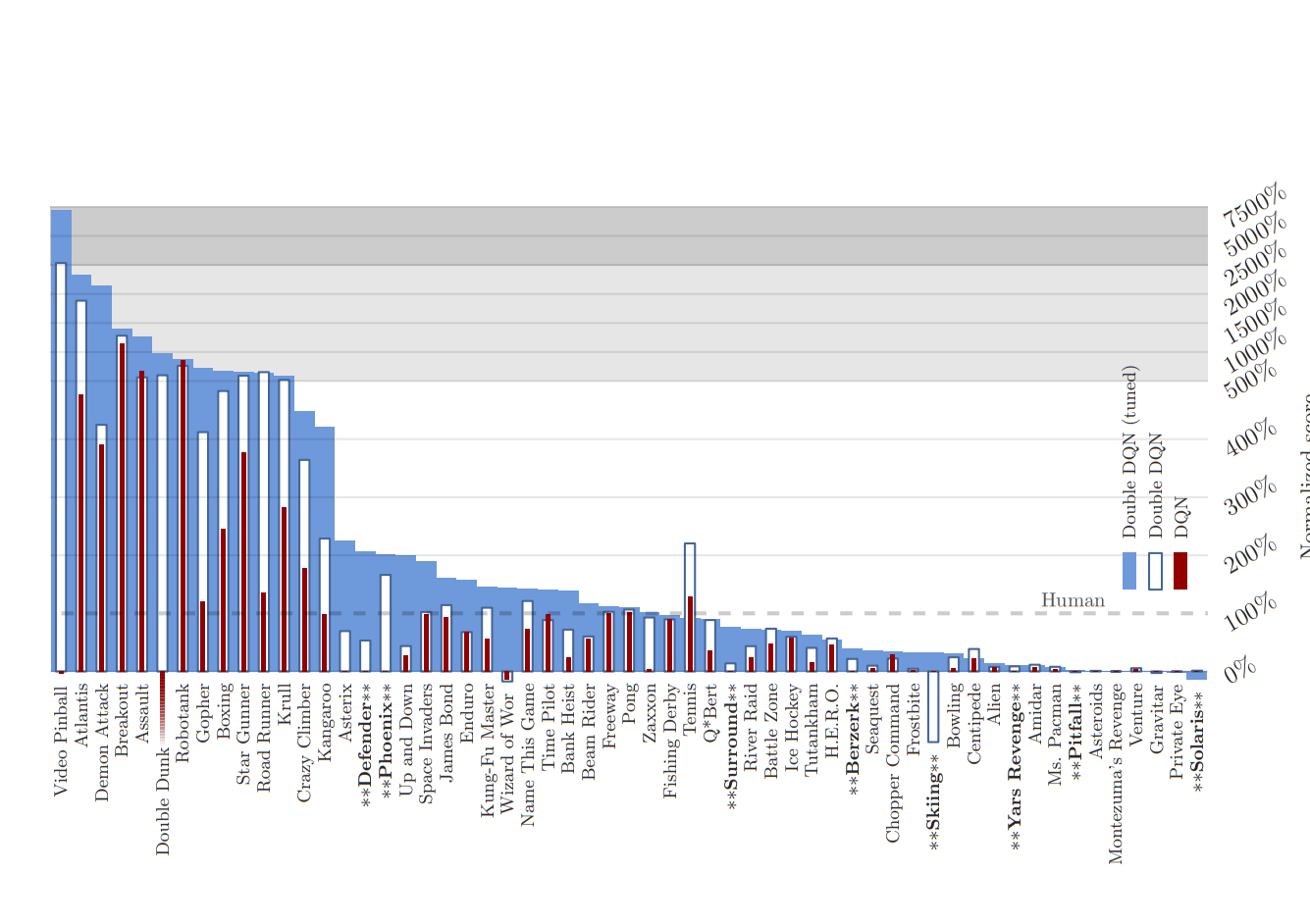
Figure 4 from van Hasselt et al. (2016) illustrates the normalized scores across 57 Atari games, comparing the performance of standard DQN and Double DQN. The results highlight significant improvements in games where Double DQN outperformed standard DQN, marked by stars and bold font in the figure. These improvements underscore the efficacy of Double DQN in achieving superior performance by mitigating the overestimation bias.

In conclusion, Double DQN represents a crucial advancement in reinforcement learning algorithms, particularly in complex environments like Atari games. By addressing the inherent bias of standard DQN, Double DQN not only enhances learning efficiency but also enables the discovery of more optimal policies.

Conclusion

Deep Q-Learning with Experience Replay is a powerful approach to mastering complex environments like Atari 2600 games. By incorporating techniques like experience replay, prioritized experience replay, target networks, and reward clipping, this method overcomes many challenges associated with training deep neural networks in reinforcement learning settings.

These innovations have been empirically validated across various Atari games, showcasing the algorithm’s ability to generalize and perform well in diverse scenarios. As research continues, further enhancements and refinements to these methods are expected, driving even more impressive advancements in artificial intelligence and machine learning.